Code
import numpy as np
import matplotlib.pyplot as plt

r = np.arange(0, 2, 0.01)
theta = 2 * np.pi * r
fig, ax = plt.subplots(
  subplot_kw = {'projection': 'polar'}
)
ax.plot(theta, r)
ax.set_rticks([0.5, 1, 1.5, 2])
ax.grid(True)
plt.show()
Anil Radhakrishnan
November 29, 2022
To develop a draft of a blog post you can add the draft: true tag to the yaml header. This will prevent the post from being published to the site.
You can add local images to the blog by: 
You can add links to other sites by: Homepage
To add python code to the site, you will need an environment with the packages installed, then you can specify jupyter: python3 in the qmd yaml .
Then, you can add python code to the blog by:

You can later refer to the figure by Figure 1
You can write in latex by: \sum_{i=1}^n a_i=0 You can even use it inline like this a_i \in \mathbb{R} \forall i.
This works for multiline complex equations as well \mathbb{1}_{\mathbb{Q}}(x)=\lim_{k \to \infty}\left(\lim_{j \to \infty}(\cos(k!\pi{x}))^{2j}\right)=\begin{cases} 1 & \text{if}\; x \in \mathbb{Q}\\ 0 & \text{if}\; x \notin \mathbb{Q} \end{cases}
You can also add citations to the blog post by “Quarto - Citations & Footnotes” (n.d.). This will be automatically added to the bibliography.
---
title: "Blogging with quarto"
author: "Anil Radhakrishnan"
date: "2022-11-29"
categories: [tutorial]
jupyter: python3
bibliography: references.bib
---
To develop a draft of a blog post you can add the `draft: true` tag to the yaml header. This will prevent the post from being published to the site.
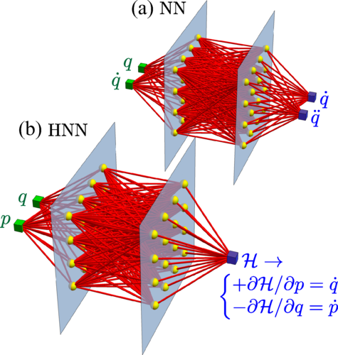
You can add local images to the blog by:
{ width=50% }
You can add links to other sites by:
[Homepage](https://webpublishing.oit.ncsu.edu/nail/)
To add python code to the site, you will need an environment with the packages installed, then you can specify `jupyter: python3` in the qmd yaml .
Then, you can add python code to the blog by:
```{python}
#| label: fig-polar
#| fig-cap: "A line plot on a polar axis"
import numpy as np
import matplotlib.pyplot as plt
r = np.arange(0, 2, 0.01)
theta = 2 * np.pi * r
fig, ax = plt.subplots(
subplot_kw = {'projection': 'polar'}
)
ax.plot(theta, r)
ax.set_rticks([0.5, 1, 1.5, 2])
ax.grid(True)
plt.show()
```
You can later refer to the figure by @fig-polar
You can write in latex by:
$$ \sum_{i=1}^n a_i=0 $$
You can even use it inline like this $a_i \in \mathbb{R} \forall i$.
This works for multiline complex equations as well
$$
\mathbb{1}_{\mathbb{Q}}(x)=\lim_{k \to \infty}\left(\lim_{j \to \infty}(\cos(k!\pi{x}))^{2j}\right)=\begin{cases}
1 & \text{if}\; x \in \mathbb{Q}\\
0 & \text{if}\; x \notin \mathbb{Q}
\end{cases}
$$
You can also add citations to the blog post by @noauthor_quarto_nodate. This will be automatically added to the bibliography.
Finally you can update the site by using `quarto render` and then `quarto publish gh-pages` to publish the site to github pages.